Since my last article (4 months ago!), my days have been filled with research, writing about the research, and presenting my research. Today I really want to do the exact same thing and write about my Master’s research project and our “Crisis in Cosmology”.

This article will be structured like my dissertation, however we will skip the big equations and overly technical details. I’ll attach my dissertation below if you’d like to have a look.

First we’ll introduce the Hubble tension and the different ways we estimate Hubble’s constant. Then we’ll look more into black hole mergers and the standard siren technique, and end with my results and conclusion.

The Hubble Tension

One of the biggest problems we’re currently facing in astrophysics is figuring out the rate of expansion of the universe, which we quantify as Hubble’s constant (or H₀). This is commonly called the Hubble Tension or the melodramatic call it the crisis in cosmology. This comes from a statistically significant disagreement in values for H₀ depending on the method used to obtain an estimate, with improvements to equipment sensitivity only exacerbating these discrepancies further.

What does statistically significant or significant mean in this case? Scientifically speaking significant means we reject the null hypothesis that what we’re seeing is chance, so there is likely something happening that’s affecting our measurements.

For example, we expect people to get disease “X” 5% of the time plus minus 2%. If we go and take a sample of hikers and found X developed in 6% of cases, it’s well within the bounds of error and our result is encompassed within the uncertainty range. That is NOT a significant result, and there’s NO evidence to suggest hiking causes disease X. If we then go and look at people who eat drywall and find they get X in 90% of cases then depending on our analysis we can say this is statistically significant result, and that drywall consumption has got something to do with disease X.

In our case, the main methods we use to determine Hubble’s constant have some uncertainty BUT they don’t overlap much. And with improvements to our equipment sensitivity we now have smaller errors but our results don’t overlap at all, and the gap is actually really big!

So we have disagreements in our results but we don’t really know why. This in turn raises another issue because we also don’t know which results are close to the actual value of Hubble’s constant, or if they’re all rubbish.

Methods

There are numerous methods in determining Hubble’s constant, however they can be split into 2 regimes: indirect and direct methods.

Of the indirect techniques, CMB measurements seem to be the only ones. This
method involves measuring the size of anisotropies in the CMB, which are expected to
accurately reflect the cosmological structure seen today in the universe. These anisotropies are just temperature fluctuations, but a little change in these fluctuations results in tremendous changes in supergalactic structures in the current universe, so they’re pretty important to study!

Hence, expansion isn’t measured by things moving away from us, but inferred from early-universe proprieties and how pressure and heat moves through the CMB.

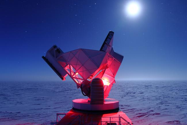
Measurements using the South Pole Telescope (SPT) estimate Hubble’s constant to be 68.8 ± 1.5 km/s/Mpc. In combination with Planck data, the most comprehensive and constrained estimate using the CMB is 67.49 ± 0.53 km/s/Mpc.

Conversely, direct methods make use of Hubble’s Law which states that the velocity of a source moving away from us, v, is directly proportional to distance to the source, d, with Hubble’s constant H₀ being the constant of proportionality:

v = H₀ d

The recessional velocity can be determined from the redshift, z, of the source using the
relation below where c is the speed of light:

v = c z

So redshift and Hubble’s law provide a very simple relationship between two observable properties (velocity and distance), but it’s the observing of these properties that causes the problems!

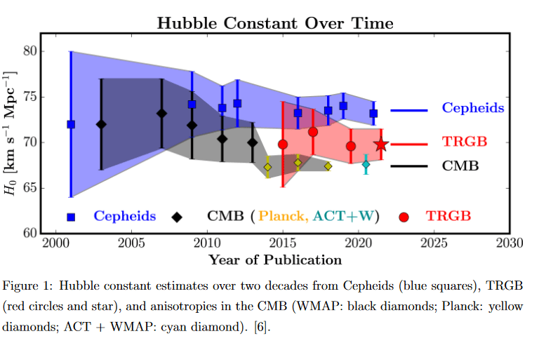
Most estimates use type 1a supernovae with their distances calibrated from either Cepheid variables or stars from the tip of the red giant branch (TRGB), so physicists usually only mention the calibrator to distinguish between the two. A recent estimate using TRGB as a calibrator found H₀ = 72.1 ± 2.0, however estimates with Cepheids tend to be slightly higher with a recent estimate of 73.3 ± 1.04.

When you compare the four results I’ve just mentioned, you’ll notice that the direct and indirect errors don’t overlap. Below is a graphic from Freedman et al which has more results over time and explains the problem better.

The Standard Siren Technique

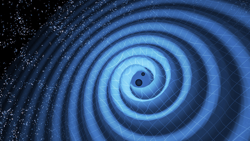
In my research, I explored the standard siren technique which uses gravitational waves (GW) instead of light to measure distances, very fancy!

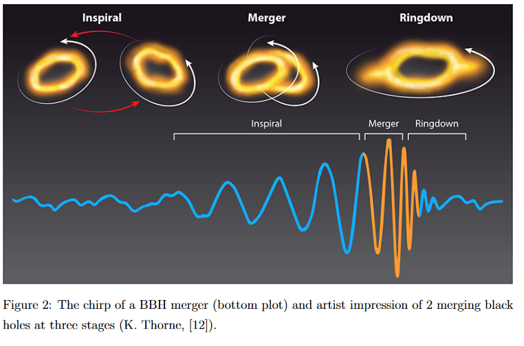
The standard siren technique is a direct method that uses binary black hole (BBH) mergers to estimate distances in lieu of distances from type 1a supernovae. Merging black holes will radiate out energy in the form of gravitational waves in order to conserve energy as they’re merging and coming closer together.

This phase is actually the inspiral, which occurs before the merging, where the separation of both black holes decrease and their orbits shrink up to the innermost stable circular orbit (ISCO). You can’t have stable orbit smaller than this, so at this distance the merging commences where both black holes combine. This ends with a newly formed black hole which gravitationally vibrates or “rings” at multiple frequencies. The ringdown is the damping of these frequencies.

Gravitational waves preserve information on mergers such as the individual masses of each black hole and their separation at each point.

What’s great is that once the masses are accounted for, the shape of the chirp (that’s the detected gravitational waves like in the above picture) is always the same but only changes in size/amplitude with distance. This means close-by mergers will have a stronger signal detected compared to more distant ones BUT The distance does not affect the general shape so we can estimate a distance by just measuring the amplitude!

Technically it’s a little more complicated than that, but that’s all the information you need to understand the concept.

Well that’s distance sorted, we just need velocity.

The location of the incoming wave cannot be determined by one detector, but you can triangulate the location with multiple detectors across the globe. Currently triangulation is completed using the aLIGO–AdV network, comprised of the LIGO Hanford detector, LIGO Livingston, and Virgo.

The reason I mention the location is because black hole mergers don’t produce any detectable light and thus we can’t find the redshift from them by themselves. However, if we know where on the sky the merger came from and the distance, we can locate from which galaxy the merger came from. Then we use the redshift of the galaxy to get a velocity.

It’s a little extra step but it works!

So why would the standard siren technique be any good? Well, I think gravitational waves may provide us with a more competitive method compared to other new methods because the target objects and technique are more independent of prior methods. While the TRGB and Cepheids produce different results, they are very similar in nature and are only a middle step in estimates using supernovae and thus may be affected by the same systematic errors just to varying degrees. This may make the standard siren technique ideal for comparing results and determining any underlying biases in certain methods. Gravitational waves are quite different to electromagnetic waves (light) and they don’t seem to have many common biases like dust extinction, so it might shed more light on the situation (no pun intended).

Current Estimates and Uncertainties

For the last part of the theory we’ll discuss the current state of estimates with gravitational waves (and yes we do have some!)

Distances uncertainties are typically 25-30% of the merger distance. I used the maximum value uncertainty (30%) for my research for the most broad range of H₀ values and errors. Thinking back, I have no clue why I did this.

When it comes to the location on the sky, the accompanying uncertainty typically expressed as a 90% credible region (CR₉₀). This is the area of the sky in which there’s a 90% chance of finding the merger. The credible region is actually hot dog shaped, which arises from the method of triangulation using multiple detectors. The picture below from B.P Abbott et al in 2018 (the one from Living Reviews Vol 21) shows this shape on a globe for the GW event GW150914.

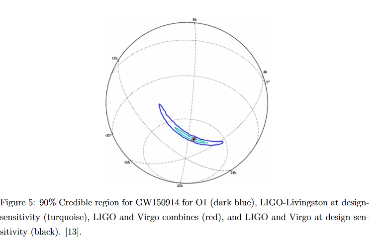
The image above shows that the CR₉₀ size has hugely decreased with each observing run and adding more detectors. The most recent completed observing run, O3, had a range of 120-180 deg², so for the locational offset I used 150 deg² as a general CR₉₀.

The earliest estimate used GW170817, the gravitational wave counterpart of a neutron star merger detected by LIGO in 2017. In this case, the host galaxy (NGC 4993) provided the recessional velocity. The final estimate of Hubble’s constant was 70⁺¹²₋₈ km/s/Mpc which fits in snuggly between previous calculations with CMB and Type 1a Supernovae. You might have noticed that I split the errors up here because they’re uneven. This will be the case for all estimates.

A following estimate found H₀ = 75.2^+39.5_−32.4 km/s/Mpc. The estimate used the luminosity distance with GW170814, and found a redshift using a nearby galaxy from the Dark-Energy survey (DES). The most recent estimate used GW190412 in a similar method, and found H₀ = 77.96^+23_−5.03 Km/s/Mpc.

These estimates seem to align quite closely to the current population of values from other methods, although they all have large uncertainties. This makes any conclusions difficult to draw from a single estimate, but one noticeable trend with each estimate is that the upper uncertainty is larger than the lower one.

I think this is from the location part, because there are loads more galaxies to choose from further from the merger than closer than the merger, meaning a GW event has a higher chance of being assigned a more distant galaxy than a closer one. This would produce an overestimate of H₀, so this is likely the cause of the asymmetrical uncertainty

Data & My Method

I won’t go into great detail of my method, otherwise this article would get too technical and long. I my also give you a headache, and potentially PTSD from vector calculus. Instead, I’ll just explain the general steps I took to create some data and get values. I’ll also publish my report in a separate section where you can read the specifics of the programming and method.

For my work, I created an artificial set of BBH mergers which closely reflect our observations and detector capabilities. These were sampled from galaxies from the EAGLE simulation, which is a handy cosmological simulation that is used to test ideas on galactic evolution.

Why did I pick a simulation as opposed to real galaxies if I want to estimate Hubble’s constant? Well, I don’t actually want to estimate Hubble’s constant, I want to test how well the standard siren technique works in determining Hubble’s constant. I can do this best if I have something solidly true that I can compare my results to. In the case of the EAGLE simulation, Hubble’s constant has been set to 67.7 km/s/Mpc (based on CMB results). So now, I have a true value of H0 to compare with, whereas with real data I could only compare my estimate with other estimates (which we don’t know are correct).

The EAGLE data (I used snapshot 28) contained positions for a couple million galaxies (an x coordinate, y coordinate, and z coordinate for every galaxy), which I trimmed down to 50’000 for the sake of my computer’s 7 year old hardware.

My first step was to create a set of mergers. With my set of galaxies, I then refined the dataset down by removing galaxies close to the edges of the simulation and those too far away (beyond a distance of around 100 Mpc). With the remaining set (I think around 30’000), I randomly selected 50 galaxies to host a merger but I made bigger galaxies have a higher chance of being selected. This is just to add a bit more realism since larger galaxies have more stars, which in turn also means they’ll have a higher chance of hosting extremely large stars which collapse into stellar black holes.

I extracted those 50 galaxy positions and created a new dataset with these coordinates. This is our dataset of mergers. However these positions match up perfectly with the host galaxy, which is just not possible with the current uncertainties in our observations.

Instead, we want to add a little noise to our positions to mimic the 30% distance uncertainty and 150 deg² uncertainty that detectors have. Each merger’s distance was increased or decreased up to 30%, the percentage amount was randomly generated. A similar process was done for the location, but this required a lot more steps to create some angles and move mergers around without changing distance.

Once distance and location were messed around with, I had a brand new set of coordinates for all 50 mergers, many were close-ish to the host, some a little less so. The plot below shows a slice of the galaxies (grey) and the mergers (green). There are a lot of mergers near the big filament at around x = 10 Mpc, which makes sense because more galaxies = higher chance of generating a merger in that general area and we cut off galaxies in the further clusters. That being said, you can probably spot 3 mergers which are wildly far away and may have just had some big uncertainties. The next and main part of the process was to estimate Hubble’s constant.

In the standard siren technique, the weakest chain in the estimation (in my opinion) is assigning the merger to it’s host galaxy. The reason I think this is because the large errors in both distance and location carry forward into this step, and it only takes one of these to be slightly off to make the wrong guess. Therefore, if I want to find the best-fit estimate for Hubble’s constant, I need the positions of the mergers and galaxies to match up really well.

Below are two different plots, the mergers are in the same position but the galaxies’ distances have increased in the left plot. This is me messing around with Hubble’s constant, and finding the ideal range of trial values of H₀ to test in my next step, but it also shows the concept really well.

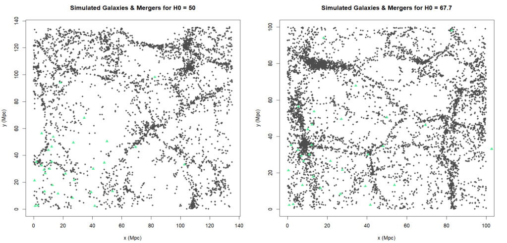
The mergers and galaxies in the left plot don’t match up well at all, in fact it appears as though all the mergers were generated in a void. The probability of Hubble’s constant being 50 is really low. Whereas on the right, the positions match up pretty well, which makes sense because 67.7 is the true value of Hubble’s constant in this simulation.

In order to test this in a more scientific way, I created a program that quantifies how well the positions match up (formally called a cross-correlation function). All this program does is find the probability that a merger originated from a galaxy based on how far away they are from each other, which is repeated for every galaxy and every merger and all these probabilities are added up to give me one final value that I called Φ (Phi). So only galaxies that are really close to a merger will have a high probability. However if there are no galaxies nearby (like in the left plot above), overall the probabilities will be low.

I ran this program for 5 values of Hubble’s constant (50, 60, 70, 80, 90), and then I made 9 more samples of 50 mergers and did the whole thing again! It took 50 hours just to run the final cross-correlation function!

Results

So now for the results. In total, I collected 50 Φ values and plotted them in this funky rainbow graph.

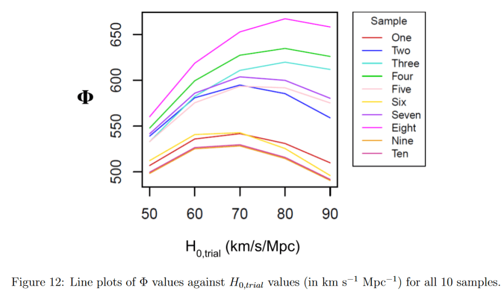
Initially, I didn’t really think anything much about the fact that the lines has different peak heights and just averaged them out like this. This was wrong, I normalized them all and then took averages which is plotted below. I also found that all the data points fit a parabola best, which was really weird since I’m used to everything fitting a Gaussian bell curve. I might just need to run the simulation below 50 and above 90 to get the tails.

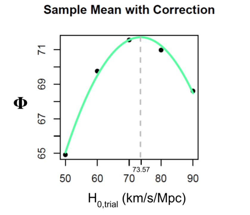
As you can see, our best H₀ value (the peak of the graph) is 73.57 km/s/Mpc. I’m actually very proud of myself for getting a result that’s similar to other results, especially since Hubble himself got an estimate of 500 km/s/Mpc because he forgot to check his axes! I would never do that!

I also did some uncertainty analysis to obtain some errors, and got a final result of 73.57 ± 3.83 km/s/Mpc.

Discussion

Right off the bat, we can concretely say that our final estimate is an overestimate. Interestingly, merger sample 6 was the only sample which was an underestimate (I plotted all 10 samples individually as well), so clearly we have a bias in our results that I didn’t factor out.

Also I managed to get identical results for samples 9 and 10. I checked the matrices of results after they ran, the values are all indeed different but through sheer coincidence their peaks ended up the same!

So overall our result is actually very close to supernova estimates as opposed to CMB ones. Some individual samples agree better with CMB measurements, and my results are in agreement with other black hole merger results but they have huge uncertainties.

The problem is that we know Hubble’s constant in EAGLE is 67.7 so we have a roughly 6 km/s/Mpc overestimate here even when I normalized all the lines. The bigger problem is also that our estimate’s uncertainty doesn’t include 67.7. This suggests our high value isn’t just a random little bit of poor luck when randomly generating the mergers, but an actual bias that we didn’t account for when running the program.

We could have just unluckily got more overestimates than underestimates, which I expect to be a 50/50 split. However, I did a binomial test and the probability of getting a 90/10 split between overestimates and underestimates turns out to be less than 1%. So I’d say this is not just a fluke and there is definitely something screwing with the samples.

I expect that the overestimate is caused by there being too many galaxies further away from the mergers than there are galaxies close-by. Even if all these distant galaxies has very low probabilities, a thousand low probabilities can add up to a noticeable amount. Thus, I think my Φs are being heavily dominated by distant galaxies.

We could remove really far galaxies from the dataset to give the closer ones a better fighting chance. The problem is that the mergers’ distance uncertainties are 30%, meaning distant mergers have much higher absolute uncertainty. For example, 30% of 10 Mpc is only 3, but 30% of 100 Mpc is 30 which is 10 times greater than the Local group. If the merger were generated in a dense patch, that’s a lot of potential galaxies encompassed within that 30Mpc, meaning we could accidentally remove the host galaxy and that would introduce an even worse bias.

If we were to do that, we’d have to go on a case-by-case basis for each merger. This is computationally too expensive because you’d be making a bespoke set of galaxies for every merger.

I think the best thing is to improve the equipment. My samples are based on high uncertainties, but they’re real and actual errors. If LIGO, Virgo, and KAGRA could get their distances down to below 15% and credible regions below 100 deg², I’d have a much easier time getting back that 67.7 km/s/Mpc.

Also, I think we need to address the elephant in the room. If our results match supernovae ones, but we know our results are overestimates, does that mean supernovae estimates are also overestimates? The short answer is that my results don’t prove anything about the validity of other methods. The standard siren technique and the supernovae techniques are fundamentally completely different methods that share Hubble’s Law as their common feature. We can’t really make conclusions on one method and expect them to fit the other, even in this case where we are just talking about the estimates being right. It also heavily depends on how well the EAGLE simulation matches with real life galaxies and whether it’s appropriate to use the CMB estimate for Hubble’s constant in the first place!

It could also be the case that all three techniques are overestimates. It would be interesting to use a simulation that is based on supernova estimates, and to also use real life data. My predecessor did this and got an estimate of around 74-75 if I remember correctly. At the end of the day, better equipment will hopefully fix this (even though it didn’t for the first two methods and made things worse).

Conclusion

In conclusion, I tested out the robustness of the standard siren technique and found it could work decently well with a large dataset and the current detecting capabilities! I generated a sample of mergers based on real life measurements and got a H₀ value of 73.57 ± 3.83. It’s a pretty good estimate, but an overestimate at that. Next steps forward are to get governments to fund gravitational wave detectors!

The weakest link appears to be assigning of the merger to the galaxy. It would be really ideal if we didn’t have to do that and could get the redshift some other way. This is why binary neutron star mergers (like BBH mergers, but neutron stars) are quite interesting, because they can release gravitational waves and a kilonova/gamma ray burst which gives us spectral data and hence a recessional velocity. The problem is we don’t see neutron star mergers often AND we’d need to see both the gravitational wave and kilonova plus correctly link the two to the same event. That could be a challenge. If you’d like to learn more about these specific events, I’d recommend papers from my supervisors Nial Tanvir, Paul O’Brien, and the honorable Phil Evans. Every paper they publish is such a great read, and have so much good information!

Overall I think the standard siren technique is a really promising method and could be a great avenue for solving the Hubble Tension. We’ll see in a few years!